Post-training
Post-training language models for scientific simulation
Learning to write reliable simulations from physics feedback
Many engineering decisions about the physical world rest on simulation. How heat moves through a battery, how a coating degrades under repeated load and how air flows over a wing are all answered by programs that advance a set of equations in time. Simulation is also how ideas are tested between slow, expensive physical experiments. Writing such a program well is a scarce skill: the method has to be accurate, stable and fast for the specific equation, and dozens of small details have to be right. The simulation a decision needs often does not exist yet, because the equation, the coefficients or the operating conditions are new.
Physics also makes that skill checkable. A solver either reproduces a trusted simulation or it does not, so its output can be scored automatically. Problems can be generated without limit, so compute, not human labeling, bounds the supply of training signal. That makes simulation a natural domain for scaling language models with reinforcement learning on verifiable rewards, the approach behind recent gains in math and code.
I post-trained Qwen3.5-9B with reinforcement learning against a physics verifier. For each problem the model writes a Python solver, a sandbox runs it, and the verifier compares the output with a reference solution. An answer counts only if its error stays below 1%.1 The model never sees a correct program. After 256 steps, pass@1, the share of single attempts that pass, rose from 9.0% to 55.7% on ten equation families held out from training. That puts a 9B model ahead of GLM-5.3 (49.1%) and MiMo-V2.6-Pro (45.6%), two far larger open-weight models with reasoning enabled, and behind Qwen3.8-Max (69.2%). Two evaluation sets, generated and sealed before training passed step 160, confirmed the gains made after that step.
What did post-training teach the model? A widely discussed result argues that reinforcement learning with verifiable rewards mostly makes a model reliable at what it could already do occasionally, rather than giving it new capabilities.2 Physics is a clean test of that claim, because a 1% error bar cannot be met by luck and the same numerical methods recur across many different equations. Within 64 samples per problem, my results support the claim in this domain. Training made the model reliable, taught it which method suits which equation, and made its answers clean enough that the governing equation can separate right from wrong.
One held-out Allen–Cahn problem, chosen because my model solved it in 8 of 8 attempts and the base model in 0 of 8. Left to right, the reference solution, my model’s first correct program and the base model’s most accurate program, with the error of each over time.
Key findings
- Post-training produced a strong solver that transfers to unseen equations. On ten held-out equation families, pass@1 rose from 9.0% to 55.7%, and on new problems from the training families it rose from 6.6% to 47.3%. Sealed sets confirmed improvement on both from steps 160 to 256 (p < 10⁻⁶).
- Most of the gain is reliability, which a reference-free check can exploit. With 64 samples the base model solves 85.2% of held-out problems at least once; my model passes that mark with eight. Choosing among eight samples by how well each satisfies the equation, a check that needs no reference, is correct on 87.8% of held-out problems, about one point below Qwen3.8-Max (89.0%) and GLM-5.3 (88.9%) with the same selection.
- Training reinforced method selection, and the largest gain followed targeted data. The model learned to use exact solutions where they exist and adaptive time integrators elsewhere, and both habits transferred to new equations. The largest jump of the run came during a phase of training problems aimed at its most common bug.
Task, verifier and training recipe
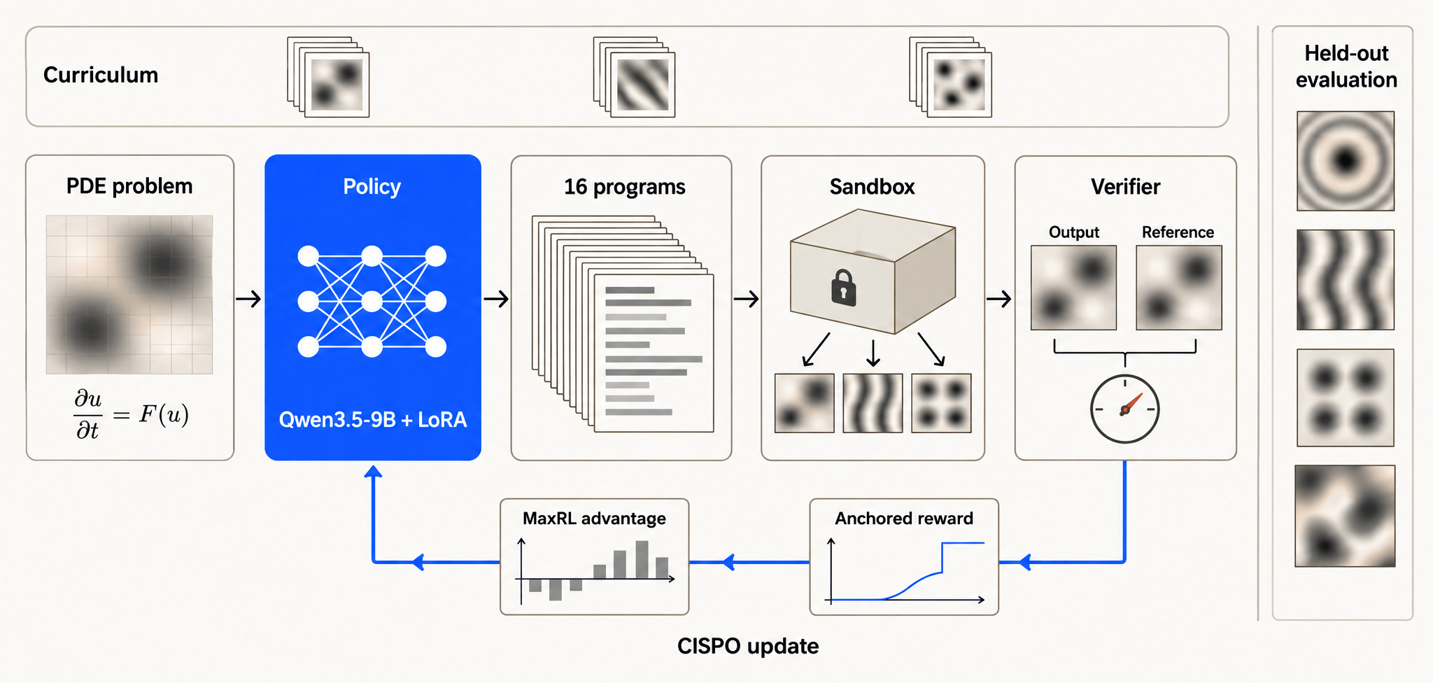
Each step samples 16 programs per problem, runs them in a sandbox and scores them against a reference. The scores become a policy update. A curriculum selects the training problems, and ten equation families are reserved for evaluation.
Task. Each problem specifies a partial differential equation,3 its coefficients, a grid, an initial state and the output times. The model writes one Python function that returns the solution at every output time, using NumPy and SciPy. Problems follow the procedures of RLVP, which introduced reinforcement learning against a physics verifier for this task.4 Training began with eight equation families and added three linear families in the final phase. Ten evaluation families, ranging from heat flow and transport to the Korteweg–de Vries and Cahn–Hilliard equations and two-dimensional pattern formation, never appear in training.
Verifier. Each program runs in an isolated sandbox with a 30 second limit on two CPU cores. Its output is compared with a reference computed by two independent methods. An answer passes only if it runs, returns the right shape and stays within 1% error.
Recipe. Two earlier attempts that followed RLVP’s recipe produced no measurable gain. Replaying every failed program with its error messages pointed to five changes.
- Base model initialization. Supervised fine-tuning on teacher solvers made the model four to ten times less accurate, because it copied the teachers’ habits, including internal labels passed to library functions as if they were method names.
- Anchored reward. Under RLVP’s reward, 76% of all credit went to programs no better than a trivial answer such as returning the initial state. My reward is zero at the best trivial answer, rises with log-error above it, and reserves half its credit for meeting the 1% bar.
- Explicit grid conventions. At a 1% bar, a model that guesses where the grid points sit fails regardless of its numerics, so each convention went into the problem statement after I checked it against the reference code.
- MaxRL advantages. A program’s advantage is its reward minus the group mean, divided by the group mean plus a stabilizing constant of 0.01.5 This gives programs that outperform their group greater weight when the group’s average reward is low.
- Adaptive curriculum. Training ran in eight phases of 32 steps. Between phases I revised the problem mix using the current model’s rewards and failure patterns, introduced fresh cases, and added three linear families in the final phase.
I used NeMo RL’s asynchronous setup, which overlaps rollout generation with learning to keep both GPUs busy, and a CISPO loss. CISPO corrects for the difference between the policy that generated a token and the current learner, capping the importance weight at five to limit how strongly a mismatch can amplify a token’s contribution to the loss. MaxRL sets each program’s advantage, and CISPO applies it in the token-level policy loss.
| Setting | Value |
|---|---|
| Policy | Qwen3.5-9B with a rank 32 adapter,6 86.6M trainable parameters |
| Algorithm | Asynchronous group policy optimization, CISPO loss, advantage normalized by the group mean |
| Steps | 256, in eight phases of 32 |
| Problems per step, samples per problem | 8, 16 |
| Learning rate | 1e-6 for the first step of each phase, then 1e-5 |
| Generation | Temperature 0.7, at most 9,216 tokens, no thinking mode |
| Compute | Two H200 GPUs and a 16-core verifier, 26 hours |
Evaluation. Every checkpoint was scored on two fixed sets with identical problems and sampling seeds. The in-distribution set has 288 new problems from six of the training families, and the held-out set has 135 problems from the ten held-out families. I estimate pass@1 from eight samples per problem and average it with equal weight per family. Two further sealed sets of 288 and 136 new problems were generated and pre-registered before training passed step 160, and opened once, after the final checkpoint was frozen.
Results
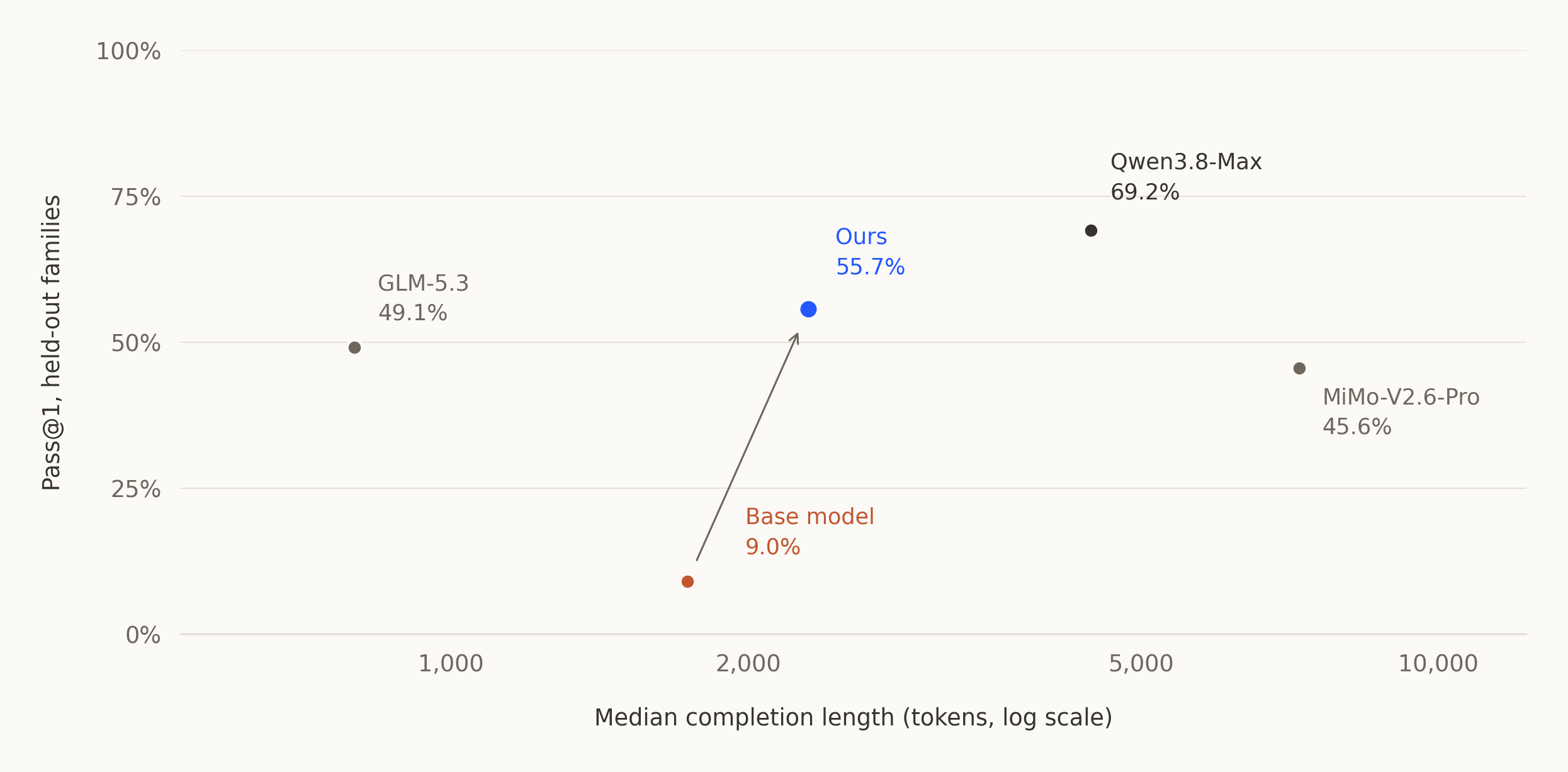
Pass@1 on the held-out families against median completion length over all eight answers to each problem, for the base model and step 256. Frontier models could use up to 32,000 output tokens with reasoning. My model generates at most 9,216 without a thinking mode.
| Held-out families, pass@1 | Overall | 1D transport | 1D higher-order | 2D transport | 2D pattern formation | 2D elliptic |
|---|---|---|---|---|---|---|
| Qwen3.8-Max | 69.2% | 93.8 | 64.9 | 82.8 | 57.6 | 0.0 |
| Ours, step 256 | 55.7% | 85.7 | 39.6 | 60.9 | 49.5 | 0.0 |
| GLM-5.3 | 49.1% | 65.0 | 25.0 | 59.9 | 62.7 | 0.9 |
| MiMo-V2.6-Pro | 45.6% | 68.0 | 12.5 | 89.1 | 24.1 | 0.9 |
| Base model | 9.0% | 16.8 | 8.9 | 5.7 | 5.3 | 0.0 |
Equal weight per family, 135 problems, eight samples each. Case-paired tests put my model 6.6 points above GLM-5.3 (p = 0.009), 10.1 above MiMo-V2.6-Pro (p = 0.005) and 13.5 below Qwen3.8-Max.
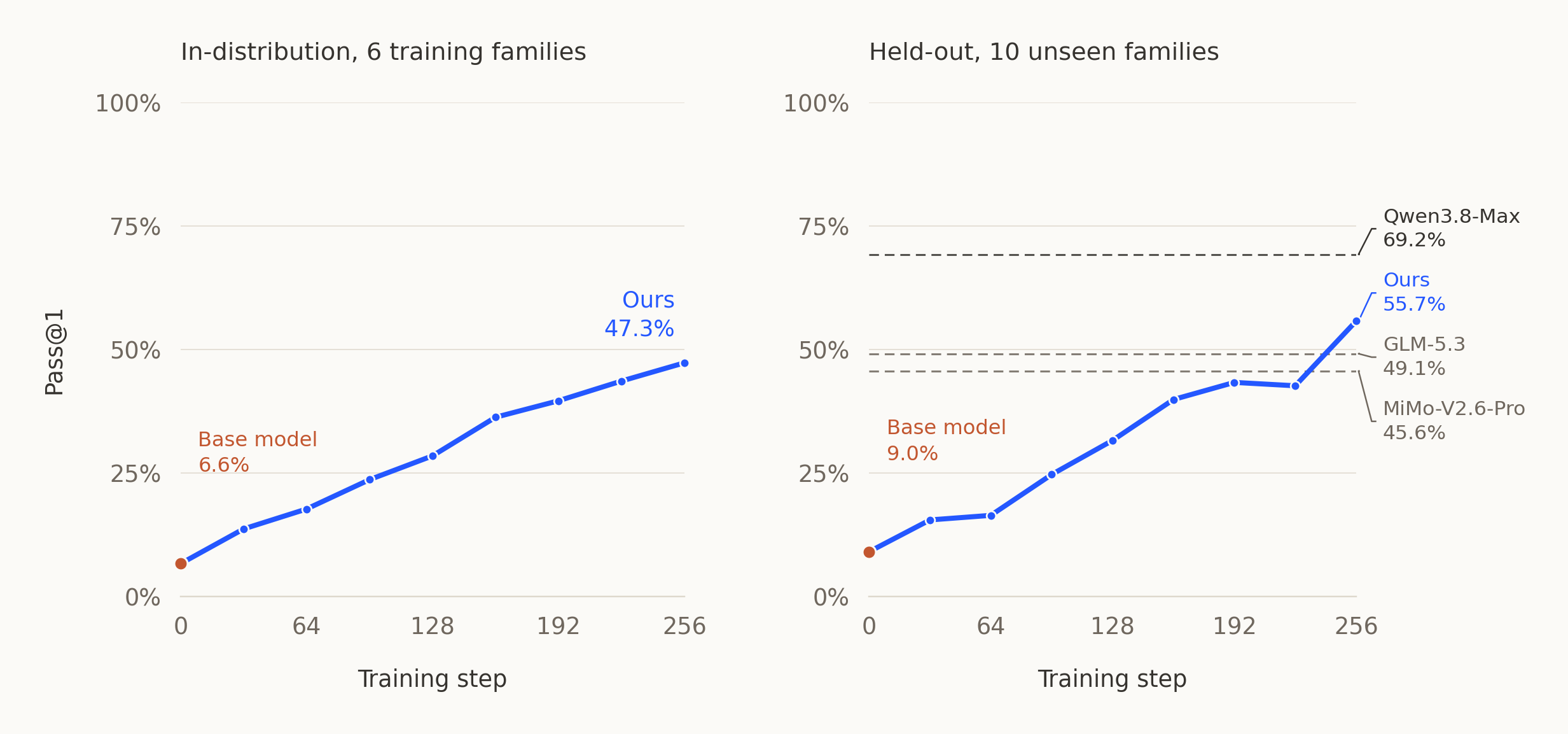
Pass@1 at every checkpoint on both fixed sets. Dashed lines mark the frontier models on the held-out families.
Both fixed sets improved through step 192. On the held-out families the phase ending at step 224 added nothing, and the final phase added 13.1 points, a jump I examine below. On the sealed held-out set the final model scored 55.3% against 41.6% at step 160, within 0.4 points of its score on the original held-out set, as the pre-registration predicted. On the sealed in-distribution set it scored 46.7% against 37.3%. Both differences hold at p < 10⁻⁶ under a case-paired test.
The model still fails on some equations. It scores zero on two-dimensional Darcy flow with a reaction term, where the frontier models score at most 0.9%, for a reason explained below. Among the other families, it is weakest on stiff nonlinear equations such as Cahn–Hilliard (29%) and Korteweg–de Vries (50%).
Sharpening versus expansion
Treat each problem as having a probability p that a single attempt passes. Then pass@1 is the average of p. Post-training can raise p where it was already above zero, which sharpens the model, or lift problems from p = 0 to p > 0, which expands what it can solve. Separating the two requires sampling the base model many times, so I drew 64 samples per held-out problem from both models.
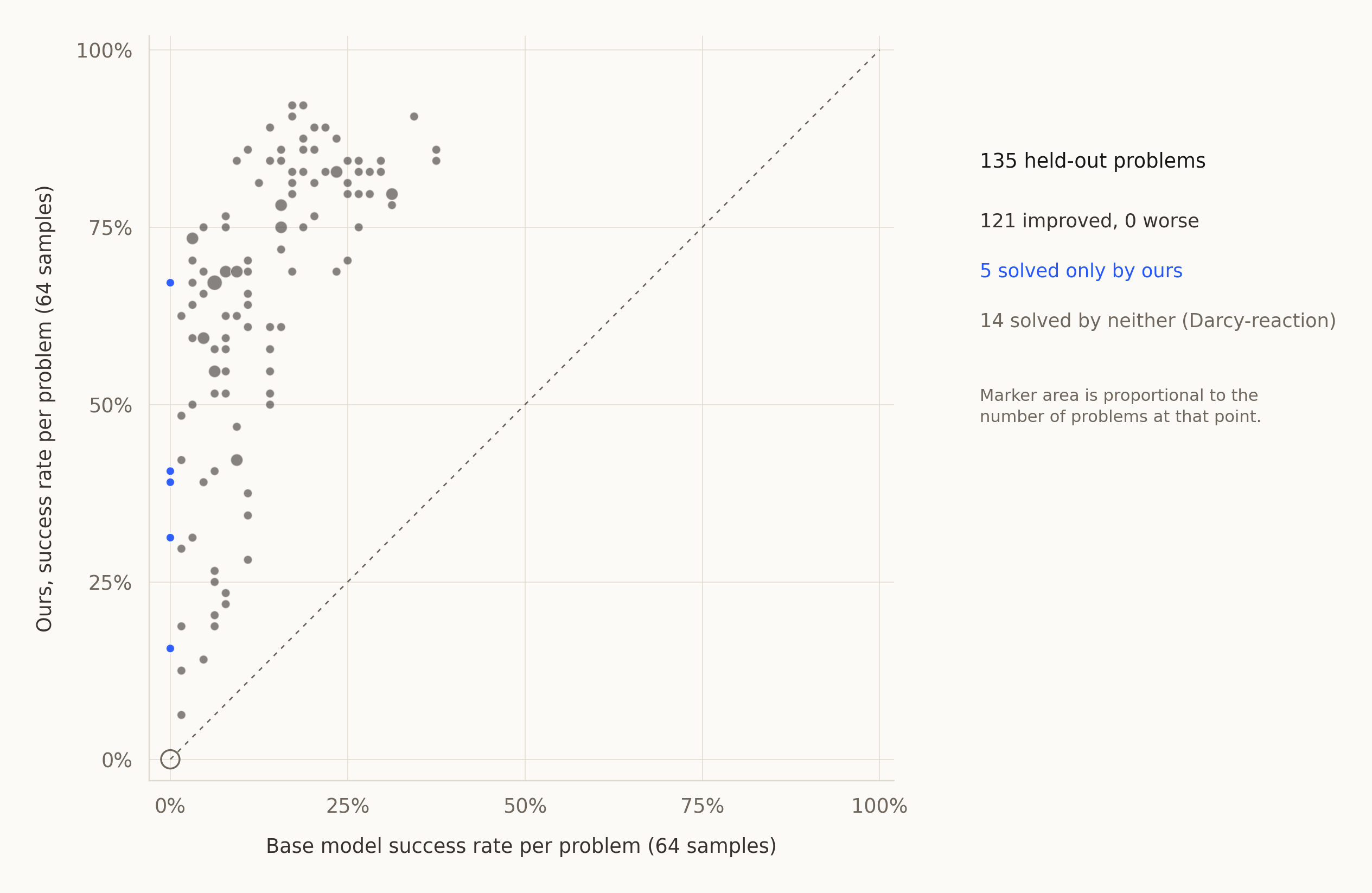
Each point is one held-out problem, with its success rate under the base model and under my model, from 64 samples each.
Most of the movement is sharpening. Of the 135 held-out problems, 121 have a higher success rate under my model and none has a lower one. The other 14 are the Darcy-reaction problems, which neither model solves. The base model solved 116 problems at least once in 64 samples, 52 of them no more than 10% of the time, and my model succeeds at least half the time on 33 of those 52. Observed reach also grew slightly. Five problems, four Gray–Scott and one two-dimensional advection, were never solved by the base model in 64 samples, and my model solves them 16% to 67% of the time.
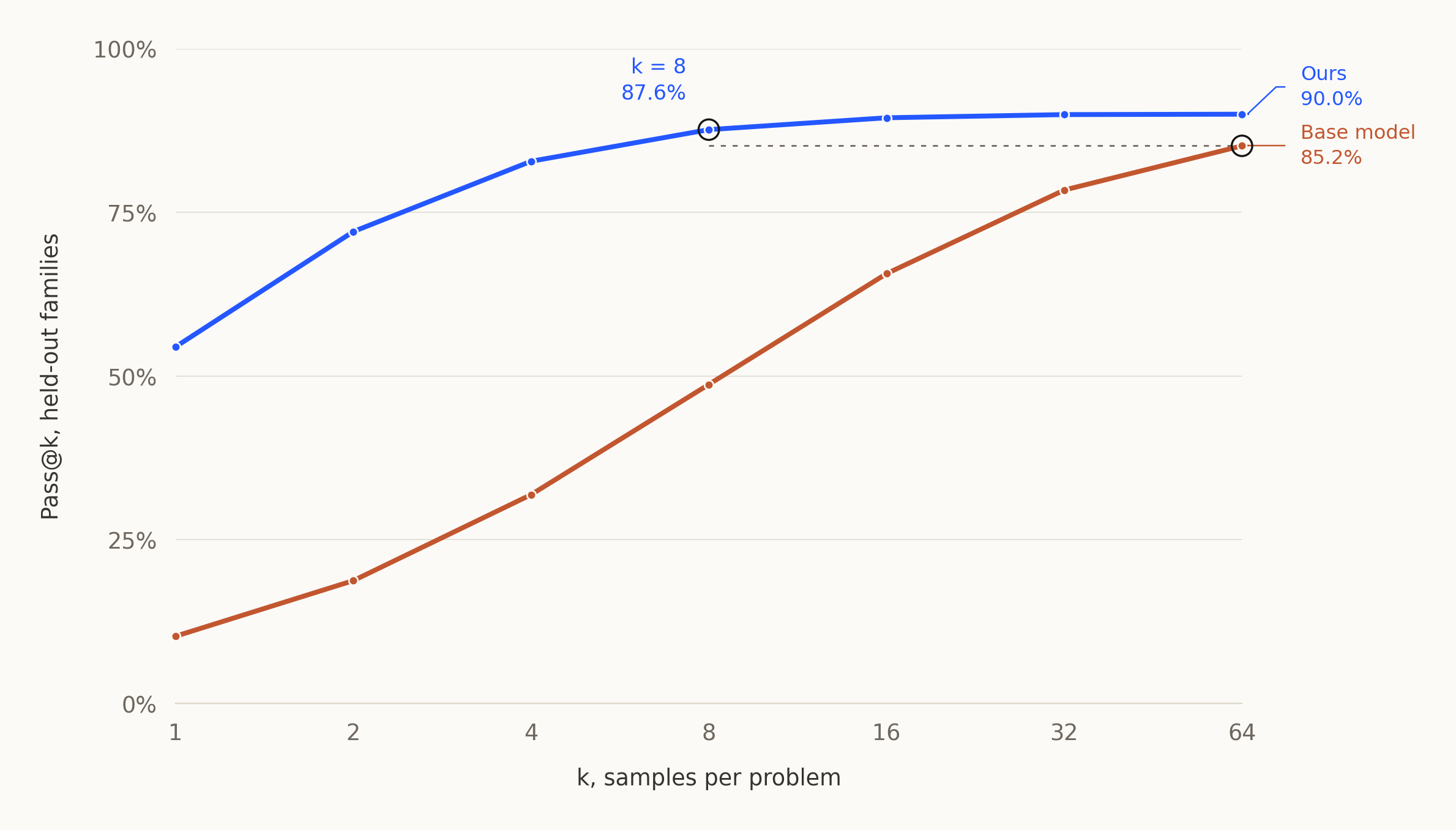
Pass@k on the held-out families, the share of problems solved at least once in k samples, estimated from 64 samples per problem. Eight samples from my model solve more problems than 64 from the base model.
The pass@k curves agree. Estimated from these 64 samples, my model’s pass@1 is 54.5%, which the base model reaches only at about eleven samples. Eight samples from my model solve 87.6% of problems, more than 64 samples from the base model solve (85.2%). The gap narrows as k grows, from 44 points at one sample to 5 at 64, the pattern Yue and colleagues reported for math and code.2 Unlike in their results, the curves do not cross within 64 samples, because of the five problems the base model never solved. Within this budget, post-training mostly concentrated probability on solutions the base model could already reach, and added a little reach on top.
Reliability matters because a model that solves a problem once in twenty attempts is useful only if you can tell which attempt was right. The governing equation offers a way: substituting a candidate solution back into it gives its residual,7 a measure of how far the candidate is from satisfying the equation, which needs no reference to compute.
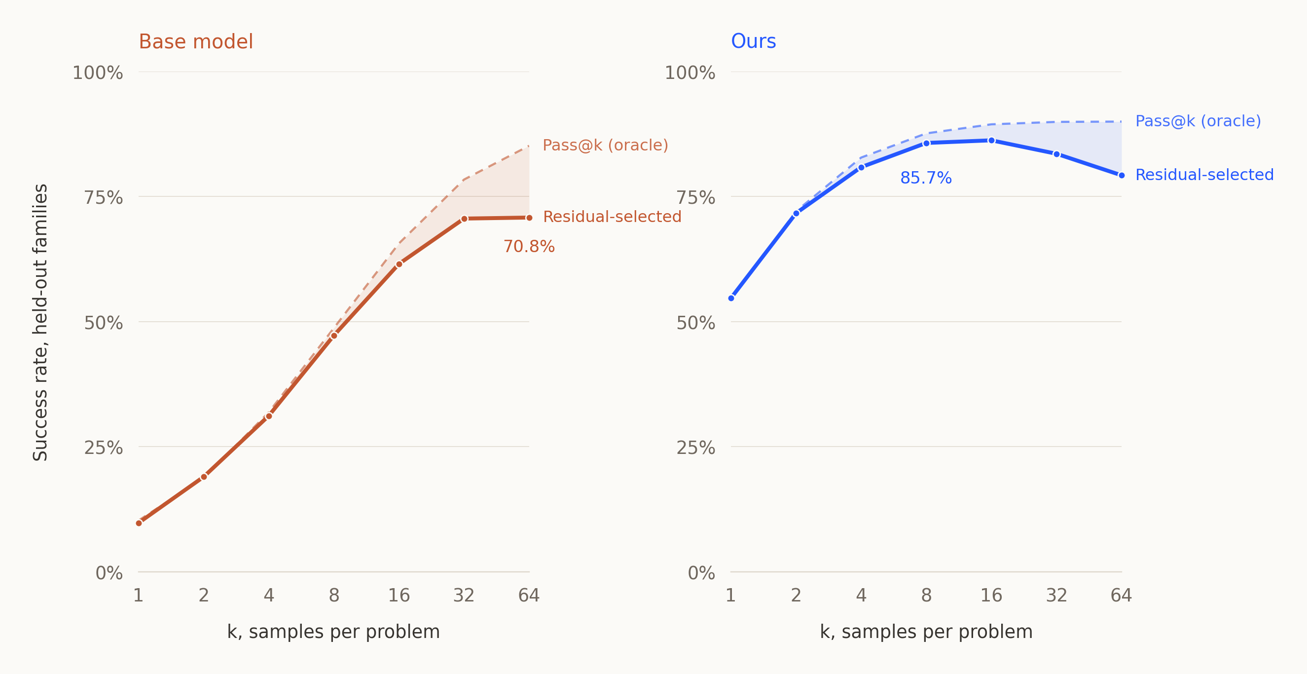
Success rate when the sample with the smallest equation residual is selected (solid) and when any correct sample counts (dashed), which requires a reference. The shaded band is what selection by residual loses.
For my model, selecting the lowest-residual answer among eight samples is correct on 85.7% of held-out problems in this analysis (87.8% in the eight-sample evaluation), close to the 87.6% that any of the eight solves. For the base model the same selection stalls near 71% beyond 32 samples, while the share solved by any sample keeps rising toward 85%. With many samples the base model produces wrong answers that nearly satisfy the equation, such as fields that barely change and ignore the starting state, and the residual picks them. Training removed most of these, but not all: my model’s residual pick peaks at 86.3% with 16 samples and falls to 79.3% at 64, because every extra sample is another chance at a wrong answer with a smaller residual. The residual check works best with a modest number of samples, and at eight it already beats 64 samples from the base model, 85.7% to 70.8%.
Learned numerical methods
To see what changed, I labeled the numerical method in every evaluation answer.8
Exact solutions. For a wave moving at constant speed on a periodic domain, the exact solution is the starting shape shifted by speed times time, and a Fourier transform9 applies that shift exactly. The base model most often stepped the wave forward in small explicit steps, which slowly smears it. By step 256 my model used the exact shift in 88% of its answers to this family, up from 11%, and those answers were correct 83% of the time.
# base model, typical              # ours, typical
for n in range(steps):              k = 2 * np.pi * np.fft.fftfreq(N, d=1 / N)
    u = u - c * dt / dx * (         u_hat = np.fft.fft(u0)
        u - np.roll(u, 1))          u_t = np.fft.ifft(u_hat * np.exp(-1j * k * beta * t)).real
Adaptive time integration. For equations without an exact formula, my model writes the spatial discretization itself and hands time stepping to a library integrator that chooses its own step sizes. On the Burgers equation10 this rose from 16% of answers to 97%. The base model often had the right idea and failed on a detail, in one case only because it returned the solution with two axes swapped.
Transfer to held-out families. On two-dimensional advection, a held-out family, the exact Fourier shift rose from 26% of answers to 97%. On the held-out Allen–Cahn equation, the adaptive integrator rose from 70% to 100%. The model learned which tool to reach for, and the same tools serve many equations.
Draft-then-final format. The model had no thinking mode, but during training it began writing a rough draft and then a clean final program, a format nothing in the reward asked for. The share of answers with this structure rose from 11% to 98%. On the in-distribution problems, median length grew from about 2,200 tokens to 4,500 and then fell to about 2,400 as the final programs became shorter.
Information per attempt. Training used about 33,000 graded rewards, each scoring a complete program. These provide a compact learning signal,11 but their number alone does not distinguish improved reliability from learning new methods. The base model already produced Fourier transforms, integrators and explicit stepping. My sampling and method analyses suggest that much of the gain came from matching these methods to equations and assembling them more reliably.
Training data and reward design
How the curriculum evolved. The first 96 steps used the original pool of 512 cases, revisiting cases with new sampling seeds. For steps 97–128, I replaced 60 training slots that had repeatedly produced only zero rewards with cases yielding larger MaxRL advantages. From step 129, I introduced fresh cases and screened advection, Burgers and one-dimensional reaction–diffusion with eight samples per candidate. I first dropped cases solved in at least seven attempts. Later screens dropped those solved in at least six, while retaining some cases with no strict pass whose graded rewards still offered a learning signal.
I adjusted the family mix between phases using training outcomes and failures on both fixed evaluation sets, including the held-out set, so held-out gains after step 224 are not a clean transfer measure. The sealed evaluation sets stayed closed until the final checkpoint was frozen, which let them check its later gains on fresh cases.
Targeted training families. Transfer stalled while the model kept improving on what it practiced. Held-out gains averaged about six points per phase through step 160, then 3.5, then none in the phase ending at step 224, even though that phase added 4 points in-distribution. Its failed programs pointed to two bugs. The most common bug in its Fourier programs was building wavenumbers for the wrong domain size, and a habit learned on one-dimensional problems, passing an axes argument to the one-dimensional transform, crashed on two-dimensional arrays. The final phase added three linear families with exact solutions, advection on domains of different lengths, the Airy equation and hyperdiffusion, which supplied problems involving domain scaling and third- and fourth-order spatial derivatives. The largest gain of the run came in that phase.
| Four linear held-out families, 496 answers | Base | Step 160 | Step 192 | Step 224 | Step 256 |
|---|---|---|---|---|---|
| Wavenumbers built for the wrong domain | 71 | 59 | 55 | 38 | 22 |
| One-dimensional transform on a 2D array | 4 | 18 | 48 | 36 | 8 |
| Correct answers | 69 | 265 | 279 | 289 | 375 |
Bug counts in the extracted programs for four held-out families: two-dimensional advection and advection-diffusion, and one-dimensional advection-diffusion and heat.8 The axes bug grew with training, then fell sharply in the final phase.
Two-dimensional advection rose from 30% to 69% in that phase. The new families share linear terms with the held-out Korteweg–de Vries and Cahn–Hilliard equations, so I treat gains there as related exposure. Excluding those two and Darcy-reaction, the remaining seven held-out families rose from 53.8% at step 224 to 68.3% at step 256. The final phase also dropped Darcy from training and shifted the family mix, and I did not run an ablation, so the attribution rests on the bug counts rather than a controlled comparison.
Partial credit on Darcy flow. On steady flow through porous rock,12 the model’s answers stalled at 3 to 8% error because of one term. The reference places the zero boundary half a cell beyond the last grid point, as the problem states, and the model placed it a full cell away. Partial credit paid for answers in that band, so the habit was reinforced. The ten correct answers it ever produced reached the right coefficient by accident. A quarter of one phase spent on this family did not move it, and every frontier model I tested makes the same mistake on the held-out variant.
Unwinnable problems. For one fluid-flow family, correct independent solvers miss the 1% bar unless they are told the exact discretization the reference used, which the problem never states. For a shock-forming regime of the Burgers equation, no solver I tried passes. I removed both from training. A benchmark with a strict bar has to check that its problems are winnable.
Reward ablation. With RLVP’s reward in place of mine, accuracy after 32 steps stayed within the spread between two training runs. Starting from the base model, a larger learning rate for the adapter, 1e-5 rather than RLVP’s 2e-6, and precise problem statements did most of the early work.
Simulation as a domain for post-training
Few groups train models to write simulation code. As of this writing, two published systems train a model to write PDE solvers from scratch: RLVP, which this work builds on, and a diffusion language model that counts an answer as correct at 10% error.13 Most work runs a fixed model with retries, feedback or search and reports average error without a pass bar,14 and benchmarks for simulation code set bars anywhere from “the code runs” to 10% error.15 A 1% bar on families the model never trained on is at the strict end. On the same ten families, RLVP’s 7B model went from 1% to 11% pass@1 and its 14B model from 11% to 21%. My base model starts near their 14B model. The gains within each pipeline are 10 points for each of theirs and 47 for mine, although the different base models, prompts, generated cases and training setups prevent a controlled comparison of the recipes.
A model that writes correct solvers changes the role of simulation in scientific work. Today an engineer or an agent calls a fixed simulator and accepts its limits. When the model can write the solver a question requires, simulation becomes something generated on demand, for the equation, coefficients and conditions at hand. That is useful only if each generated simulation is checked before anyone acts on it. Physics supplies checks of increasing cost and fidelity, from the residual and conservation laws, which cost almost nothing, to comparison with an independent reference solution, to calibration against measurement, which anchors the rest. Each level is also a source of verified training signal. My model already works with the cheapest of these, the residual: with eight samples and residual selection it is correct on 86 to 88% of held-out problems at a 1% bar, on one GPU, in about 2,300 tokens per answer.
Three lessons seem likely to hold beyond this run. First, post-training against a verifier mostly buys reliability within the base model’s observed reach. Reinforcement learning turned a model that sometimes solves a problem into one that usually does, across equations, likely because the methods are shared. What it can reach depends largely on what the model already knows, which makes the choice of base model and the variety of methods in its pre-training data as important as the training run.
Second, verification should stay separate from generation. Training against a reference teaches the model, and a check the model does not control, such as the residual or a conservation law, is what makes its answers usable on problems that have no reference. The two depend on each other, because training made the answers clean enough for the check to work.
Third, stalled transfer is a reason to revisit the training data. My largest held-out gain followed a phase aimed at recurring failures, which suggests targeted data is worth testing before simply extending the run.
The same recipe could apply wherever a simulation can be checked, and molecular dynamics is a natural next domain. Agents that set up and run molecular simulations exist, but they run fixed models, the best solves about a fifth of easy tasks in a recent benchmark, and some report results they never computed.16 The one reinforcement learning system I found grades correctness with another model’s rubric rather than physics. Molecular dynamics has physical checks of increasing cost, from energy drift and momentum conservation to density and radial distribution functions against a reference. Each simulation domain with a cheap, strict check is a candidate environment for improving a model’s scientific capability with reinforcement learning as compute grows, provided each check pins down the conventions it depends on, as the Darcy result shows. Without that, training learns to satisfy the check rather than the physics. Such training should aim for the kind of skill that transferred here, a way of solving rather than a set of answers, because the next problem is rarely in any training set.
Limitations
- One training run. The 256-step run is a single seed. An independent replication covered only the first 64 steps, where both gains reproduced.
- Pre-registered and exploratory results. The sealed comparisons were pre-registered. The 64-sample analysis, the method labels and the attribution of the final phase are exploratory.
- Frontier comparison. Frontier models were scored once, with one prompt, by my verifier, with more output tokens and reasoning enabled. Their results were frozen before my final checkpoint existed.
- Scope. All problems are one- or two-dimensional on structured grids, with a 1% bar, a 30 second limit and NumPy and SciPy only. Three-dimensional flow, complex geometry and multiphysics are untested.
- Residual selection. The residual is computed on the output grid and does not check initial or boundary conditions, so it can prefer answers that satisfy the equation but violate them. Its accuracy falls as the number of samples grows beyond about 16.
Open questions
- Expansion at larger budgets. My model solves five problems the base model never solved in 64 samples. Sampling the base model hundreds of times would test whether this gap in observed reach persists at larger budgets, as Yue and colleagues investigated for math.
- Implicit and exponential methods. Can targeted problems teach the implicit and exponential methods that stiff nonlinear equations need, or does that require demonstrations from a stronger model?
- Residuals as a reward. With initial and boundary conditions added, the residual could reward answers on problems that have no reference solution.
The trained adapter is available at huggingface.co/Jarrodbarnes/qwen3.5-9b-pde-solver. The code, verifier and evaluation pipeline are at github.com/jbarnes850/pde-solver-rl.
@misc{barnes2026pdesolver,
  title  = {Post-training language models for scientific simulation},
  author = {Barnes, Jarrod},
  year   = {2026},
  url    = {https://jbarnes850.github.io/2026/10/12/post-training-language-models-for-scientific-simulation/}
}
-
The root mean square difference from the reference, divided by the range of the reference, over all output times. ↩
-
Yue et al., “Does reinforcement learning really incentivize reasoning capacity in LLMs beyond the base model?” (arXiv 2504.13837, NeurIPS 2025). They compare models with up to 1,024 samples on math, code and visual reasoning and find the base model catches up as samples grow. ↩ ↩2
-
A partial differential equation describes how a quantity, such as temperature or concentration, changes across space and time. The heat equation is the classic example. ↩
-
Cai, Utkarsh, Edelman, Rackauckas and Gómez-Bombarelli, “Reinforcement Learning with Verifiable Physics. Post-training LLMs with Continuous Rewards” (arXiv 2607.10474). I regenerated problems for the same ten held-out families with the same 1% bar and scoring. Base models, prompts and training differ. ↩
-
This follows maximum-likelihood reinforcement learning (arXiv 2602.02710). Its extension to non-negative graded rewards motivates optimizing the log of expected reward. I use mean-normalized advantages with a stabilized denominator and CISPO. This run does not isolate their effect from the other recipe changes. ↩
-
A low-rank adapter is a small set of extra weights trained on top of the frozen model. ↩
-
Zero means the solution satisfies the equation exactly. The residual here is computed on the verifier’s grid and does not check initial or boundary conditions. ↩
-
Method and bug labels are static pattern matches on the extracted program with comments removed. I spot-checked them by hand, but they are not exhaustive. ↩ ↩2
-
A Fourier transform rewrites a periodic signal as a sum of waves. Shifting each wave by the right phase shifts the whole signal exactly. ↩
-
A simple model of a fluid in which faster parts of a wave overtake slower ones and steepen it. ↩
-
This follows the information argument in Thinking Machines, “LoRA Without Regret” (2025). ↩
-
Darcy flow describes fluid seeping through a porous material such as soil or rock. ↩
-
DiffPDE (arXiv 2608.30532) trains a diffusion language model with a repair step and counts a solver as correct at 10% error. ↩
-
For example CodePDE (arXiv 2505.08783) and PDE-SHARP (arXiv 2511.00183). ↩
-
For example MooseBench (arXiv 2605.09360), which checks that the intended equations are set up, and fluid and finite-element benchmarks that pass answers within 10%. ↩
-
MDCrow (arXiv 2502.09565) and MDGym run fixed models. MDAgent2 (arXiv 2601.02075) trains with reinforcement learning on LAMMPS tasks using a rubric scored by another model. ↩